The model

We begin by describing the simplest version of our model. Later on, we will introduce several modifications, in order to deal with time dependent parameters.

Consider a hidden process (the non-observable actual number of counts in the phenomenon under study) $X_n$ with Po-INAR(1) structure:

(1) $\begin{equation*}X_n=\alpha \circ X_{n-1}+W_n(\lambda),\end{equation*}$

where $0<\alpha<1$ is a fixed parameter, $W_n \sim$ Poisson( $\lambda$ ), i.i.d., independent of $X_n$ are the innovations, and $\circ$ is the binomial thinning operator: $\alpha \circ X_{n-1}=\sum_{i=1}^{X_{n-1}}Z_i$ with $Z_i$ i.i.d Bernoulli( $\alpha$ ) random variables. Later on, we shall introduce time dependence, and hence we will be considering that $\lambda$ is a funtion of $n$ .

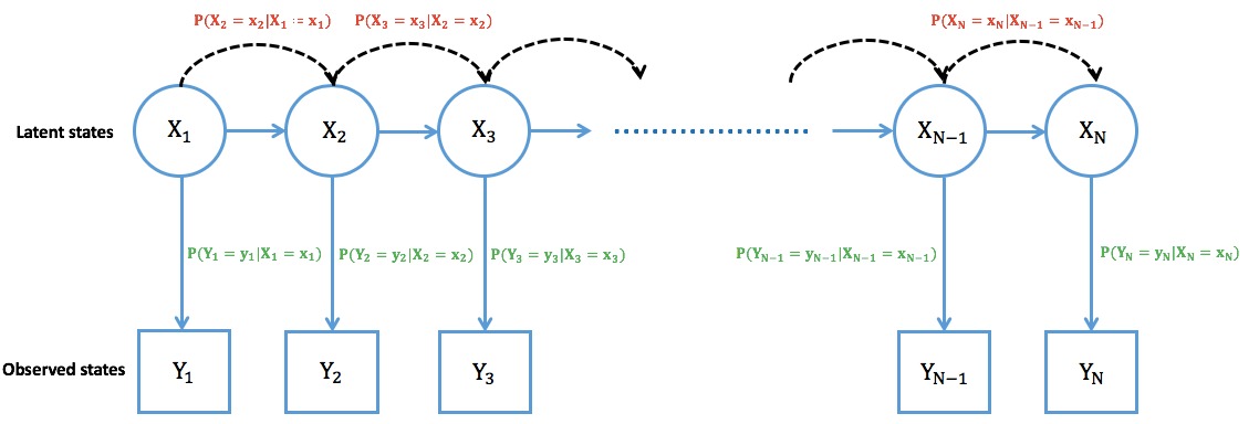
The INAR(1) process is a homogeneous Markov chain with transition probabilities

$\mbox{\bf P}(X_n = i | X_{n-1} = j) = \sum_{k=0}^{i\wedge j} {j \choose k} \alpha^k (1-\alpha)^{j-k}\mbox{\bf P}(W_n=i-m)$

The expectation and variance of the binomial thinning operator are

$\textrm{{\bf E}}\left(\alpha \circ X_{n-1}|X_{n-1}=x_{n-1}\right)=\alpha x_{n-1}$

$\textrm{{\bf Var}}\left(\alpha \circ X_{n-1}|X_{n-1}=x_{n-1}\right)=\alpha (1-\alpha)x_{n-1}$

A simple under-reporting scheme

The under-reported phenomenon is modeled by assuming that the observed counts are

(2) $\begin{equation*}Y_n = \left\{ \begin{array}{ll} X_n & \text{with probability } 1-\omega\\ q \circ X_n & \text{with probability } \omega, \end{array} \right.\end{equation*}$

where $\omega$ and $q$ represent the frequency and intensity of the under-reporting process, respectively. We will eventually be interested in considering that $q$ is time dependent: $q_n$ . That is, for each $n$ , we observe $X_n$ with probability $1-\omega$ , and a $q$ -thinning of $X_n$ with probability $\omega$ , independently of the past $\{X_j: j \leq n\}$ .

Hence, what we observe (the reported counts) are

$Y_n = (1- \mbox{\bf 1}_n)X_n + \mbox{\bf 1}_n \sum_{j=1}^{X_n} \xi_j \quad\quad \mbox{\bf 1}_n\sim\mbox{Bern}(\omega), \quad \xi_j\sim\mbox{Bern}(q)$

Properties of the model

The mean and the variance of a stationary INAR(1) process $X_n$ with Poisson( $\lambda$ ) innovations are $\mu_X=\sigma_X^2=\frac{\lambda}{1-\alpha}$ .
Its auto-covariance and auto-correlation functions are $\gamma_X(k)=\alpha^{|k|}\lambda$ and $\rho_{X}(k)=\alpha^{|k|}$ respectively.
Hence,

(3) $\begin{equation*} \mbox{\bf E} Y_n =\mbox{\bf E} X_n (1-\omega(1-q)).\end{equation*}$

The auto-covariance function of the observed process $Y_n$ is

$\gamma_Y(k)=(1-\omega(1-q))^2\alpha^{|k|}\mu_X$

Hence, the auto-correlation function of $Y_n$ is a multiple of $\rho_{X}(k)$ :

$\rho_Y(k)=\frac{(1-\alpha)(1-\omega(1-q))^2}{(1-\alpha)(1-\omega(1-q))+\lambda(\omega(1-\omega)(1-q)^2)}\alpha^{|k|}=c(\alpha,\lambda,\omega,q)\alpha^{|k|}.$

Parameter estimation

The marginal probability distribution of $Y_n$ is a \textbf{mixture of two Poisson distributions}

(4) $\begin{align*}Y_n &\sim\begin{cases}\textrm{Poisson}\left(\frac{\lambda}{1-\alpha}\right) &\quad\mbox{with probability } 1-\omega,\\\textrm{Poisson}\left(\frac{q\lambda}{1-\alpha}\right) &\quad\mbox{with probability } \omega.\nonumber\end{cases}\end{align*}$

When $q=0$ the distribution of the observed process $\{Y_n\}$ is a zero-inflated Poisson distribution.

From the mixture we derive initial estimations for $\alpha$ , $\lambda$ , $\omega$ and $q$ , to be used in a maximum likelihood estimation procedure.

The likelihood function of $Y$ is quite cumbersome to compute,

$P(Y)=\sum_XP(X,Y)=\sum_xP(Y|X=x)P(X=x)$

hence the forward algorithm (Lystig and Hughes (2002)), used in the context of HMC is a suitable option.

Consider the forward probabilities

(5) $\begin{align*}\alpha_k(X_k)=P(Y_k|X_k)\sum_{X_{k-1}}P(X_k|X_{k-1})\alpha_{k-1}(X_{k-1}) \nonumber,\end{align*}$

with $\alpha_1(X_1)=P(X_1)P(Y_1|X_1)$ .

Then, the likelihood function is

$P(Y)=\sum_{n}\alpha_n(X_n).$

$P(Y_k|X_k)$ and $P(X_k|X_{k-1})$ are the so-called emission and transition probabilities.

Transition probabilities are computed as

(6) $\begin{align*}P(X_n=x_n \mid X_{n-1}=x_{n-1})=e^{-\lambda}\sum_{j=0}^{x_n\wedge x_{n-1}}\binom{x_{n-1}}{j}\alpha^j(1-\alpha)^{x_{n-1}-j}\frac{\lambda^{x_n-j}}{(x_n-j)!} \nonumber\end{align*}$

While emission probabilities are given by

(7) $\begin{align*}P(Y_i=j \mid X_i=k) & = \left\{ \begin{array}{lcc}0 & if & k < j \\(1-\omega) + \omega q^k& if & k=j\\\omega \binom{k}{j} q^j (1-q)^{k-j}& if & k > j,\end{array}\right. \nonumber\end{align*}$

From this computations, a nonlinear optimization program computes the MLE estimates of the parameters.

Reconstructing the hidden chain $X_n$

In order to reconstruct the hidden series $X_n$ , the Viterbi algorithm (Viterbi, 1967) is used.

The idea is to provide the latent chain $X_1^*=x_1^*,\dots, X_N^*=x_N^*$ that maximizes the likelyhood of the latent process given the observed series, assuming all the parameters are known.

Let $P(X_{1:n}|Y_{1:n})$ be the likelihood function of the model, then

$P(X_{1:n}|Y_{1:n})=\frac{P(X_{1:n},Y_{1:n})}{P(Y_{1:n})}$

Since $P(Y_{1:n})$ does not depend on $X_n$ , it is enough to maximise the probability $P(X_{1:n},Y_{1:n})$ .

The hidden series is reconstructed as:

$X^*=\arg\max_{X} P(X_{1:n},Y_{1:n}).$

Predictions

Having observed $Y_1, \dots Y_n$ , we are interested in predicting $Y_{n+k}$ , for $k=1,2,\dots$ , and in evaluating the uncertainty of these predictions.

From equation 3, we have that $\mbox{\bf E} Y_{n+k} = \mbox{\bf E} X_{n+k} (1-\omega + q\omega )$ , so that, if we have a good estimate for $\mbox{\bf E} X_{n+k}$ , then we can predict $Y_{n+k}$ by means of its expectation $\mbox{\bf E} Y_{n+k}$ .

From (1), assuming that the expectation of the innovations depends on $n$ , that is, the noise is Poisson( $\lambda_n$ ) it is straightforward to see that

(8) $\begin{eqnarray*}\mbox{\bf E} X_{n+1}& = &\alpha \mbox{\bf E} X_n +\lambda_n \\ \nonumber\mbox{\bf E} X_{n+2}& = &\alpha^2 \mbox{\bf E} X_n + \alpha \lambda_n+ \lambda_{n+1} \\ \nonumber\vdots & & \\ \nonumber\mbox{\bf E} X_{n+k} & =& \alpha^k \mbox{\bf E} X_n + \sum={s=1}^k \alpha^{k-s} \lambda_{n+s-1}\end{eqnarray*}$

The easiest way to estimate $\mbox{\bf E} X_n$ is by substituting $\ Y_n$ by $Y_n$ in (3), to get
$\mbox{\bf E} X_n \approx \frac{ Y_n}{ 1-\omega + q\omega}$ , and then in 8 to get

(9) $\begin{eqnarray*}\mbox{\bf E} Y_{n+1}& = &\alpha Y_n +(1-\omega + q\omega) \lambda_n \\ \nonumber\mbox{\bf E} Y_{n+2}& = &\alpha^2 Y_n + (1-\omega + q\omega) (\alpha \lambda_n+ \lambda_{n+1}) \\ \nonumber\vdots & & \\ \nonumber\mbox{\bf E} Y_{n+k} & =& \alpha^k Y_n + (1-\omega + q\omega) \left( \sum={s=1}^k \alpha^{k-s} \lambda_{n+s-1}\right)\end{eqnarray*}$

Bibliography

T.C. Lystig, J.P. Hughes (2002), Exact computation of the observed information matrix for hidden Markov models, Jr of Comp.and Graph. Stat.

Viterbi, A.J. (1967), Error bounds for convolutional codes and an asymptotically optimum decoding algorithm. IEEE Transactions on Information Theory, 13, 260-269

Select your language

Right Sidebar